In this post I want to show you a method to solve snap-back problems in finite element analysis.
Snap-back is a convergence nightmare since cannot be easily solved by applying displacement based boundary conditions since the load-displacement curve ripples backwards!
Before getting started, you can download here all the input files of the models that we will be exploring along this post.
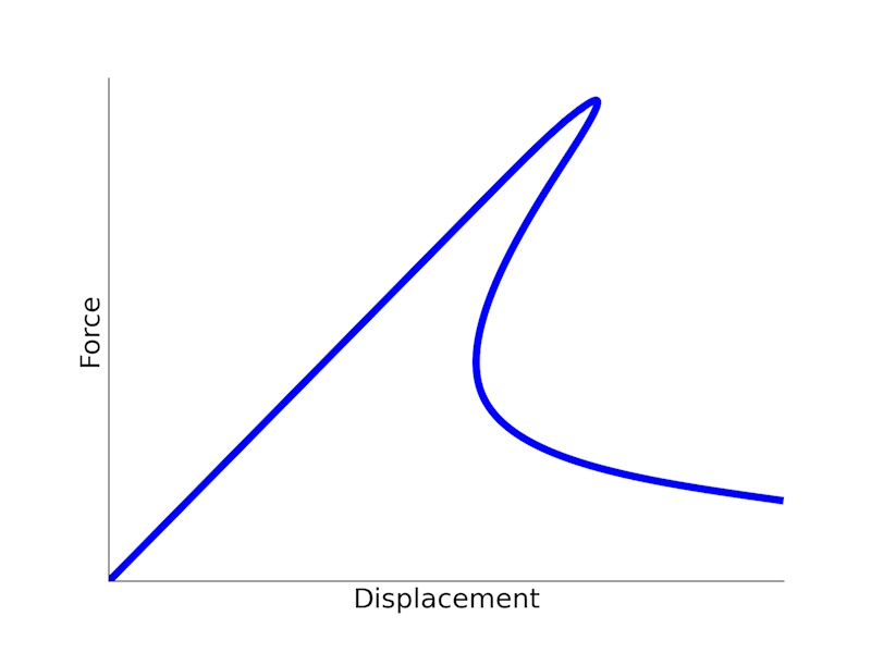
Figure 1. Snap-back takes place when the load-displacement curve goes backwards
1. Introduction
Convergence issues are one of the main obstacles to carry out successful simulations.
In Finite Element Analysis, a very common convergence problem appears when the load variable does not increase monotonically throughout the simulation. For example, when the force applied at some point decreases, we have softening! which may be caused by the material, geometrical nonlinearities, etc.
Snap-back typically takes place when the structure is loaded in such a way that it reaches a bifurcation or instability point. When that happens there is a sudden change in the deformation mode, hence “snaps”. This is clearly evidenced in buckling phenomena where there is a sudden load drop when deformation of the structure becomes bending-dominated and the load capacity falls drastically.
Simulating these phenomena through the classical displacement-based boundary condition is not enough in general. The solver will struggle to find the solution skipping the ripple (snap), especially when there is a lot of elastic energy stored in the structure at that moment.
What can we do then?
Let’s explore a general control method applicable to any FE analysis. This method is applicable to any FE software and in this post I will explain how to implement it in Abaqus.
2. The Solution
Let’s get started by defining the concept of “load variable“, this is the boundary condition that we use to introduce strains and stresses in our model. In general, this “load” is either a force or a displacement:
- Force. Applied in our FE model when we need to represent a known force/moment, a weight, wind load, etc. However, the application of forces is not recommended, as soon as the load carrying capacity of the structure decreases, the simulation will not converge.
- Displacement. The most general boundary condition to introduce load in our FE model. Applying displacements is more stable than forces because the simulation will converge even if the structure experiences softening.
The load variable is defined by the user, and therefor it must increase monotonically along the simulation. Convergence problems appear when this load variable does not increase monotonically. Snap-back takes place when the load variable is a displacement and does not increase progressively, but rather needs to roll back at the instability point.
We can minimize convergence problems like snap-back if we find a load variable that increases monotonically along the full history of the simulation.
In fracture simulations, the crack opening displacement (COD) often satisfies this condition. The key point is to make the COD the “control variable”.
The control technique that we are about to explain was proposed by J. Segurado in his Phd Thesis (section 3.5).
Let’s say that we want to simulate the double-edged notch test (DENT) shown in the figure. A uniform vertical displacement is applied on the upper edge by means of a reference point (\(L_1\)), the lower edge is clamped, and by taking advantage of the symmetry only one half of the piece is modelled (including the corresponding symmetry condition). To capture crack propagation, a layer of cohesive elements was inserted along the potential crack path.
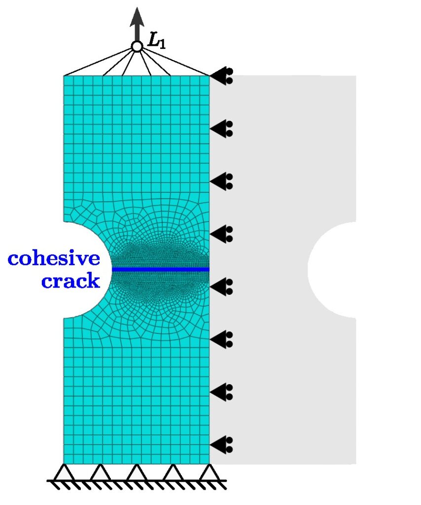
Figure 2. Schematic, mesh and boundary conditions of the DENT finite element model
This problem exhibits a very sharp snap-back triggered when the crack starts to propagate. There is no way Abaqus will solve it following standard methods. That’s why it is the perfect example to put in practice the new control method.
2.1 - Control technique
The control variable will be the COD, that will be represented as the relative vertical displacement between nodes \(C_1\) and \(C_2\):
$$COD = u_y^{C_1} – u_y^{C_2}$$
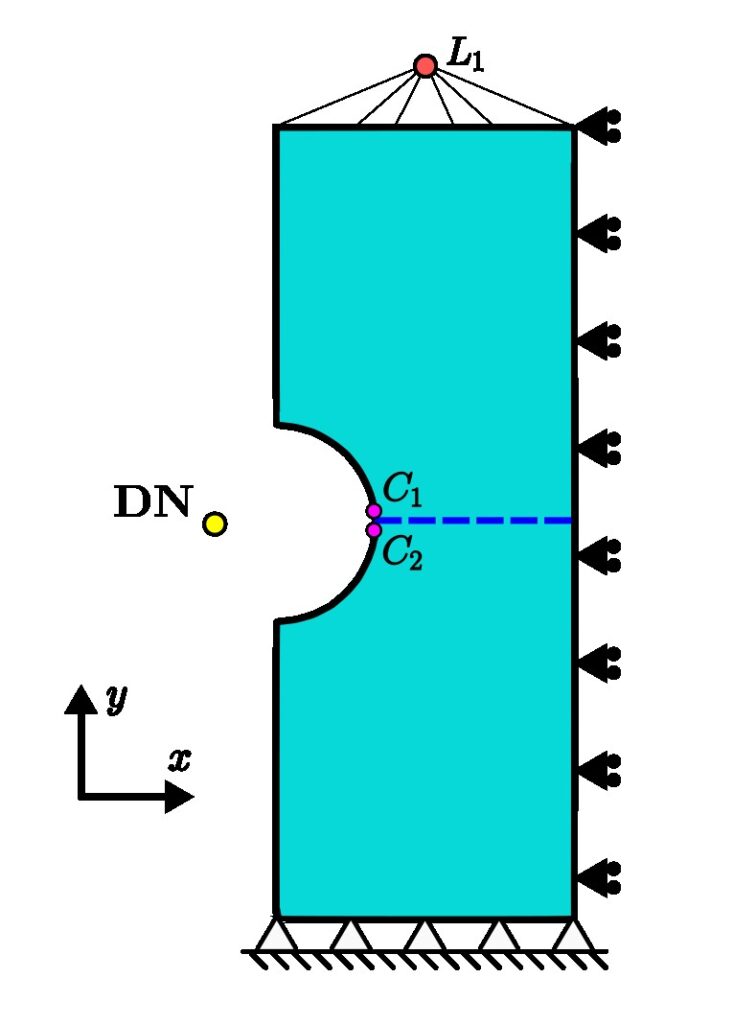
Figure 3. Location of the main nodes involved in the control technique: \(C_1, C_2, DN\) and \(L_1\).
Then, we create a director node (DN) outside of the original mesh and define the force on this node to be equal to the control variable (COD):
$$f_y^{DN} = u_y^{C_1} – u_y^{C_2} \tag{1}$$
The last step is to attach the director node to the loaded region, the reference point \(L_1\), and we will do it through the displacement:
$$f_y^{L_1} = u_y^{DN} \tag{2}$$
Finally, the load variable will be the force applied on the director node, which represents the crack opening displacement as stated through eq. (1).
It may seem that we are applying the COD directly, but that only works as a control variable, the true force is applied on \(L_1\).
3. Example 1: Double-edged notch test
Let’s see how to implement this control algorithm in the previous example: a DENT.
The input file corresponding to this example is ‘DENT_control.inp‘
First we create the director node (DN). The node location and coordinates are irrelevant, since this node will be used from an analytical perspective. Use the keyword *Node followed by the node label and x,y,z coordinates as shown below:
- inp
					*Node, nset=DN
5269, 0., 0., 0.
Quick tip!
If you are not used to working with the input file,
I encourage you to take a look at this blog post
3.1 - Custom user elements
Here comes the “meat” of this method, how to introduce the equations (1 and 2) described in the previous section. In Abaqus, we can do so by creating our own user element with a custom stiffness matrix.
a) Defining equation 1
Let’s rewrite equation (1) in FEM terms:
$$\underbrace{\begin{bmatrix}
0 & 0 & 0 \\
0 & 0 & 0 \\
1 & -1 & 0 \\
\end{bmatrix}}_{K_1}
\begin{Bmatrix}
u_y^{C_1} \\
u_y^{C_2} \\
u_y^{DN}
\end{Bmatrix}
=
\begin{Bmatrix}
f_y^{C_1} \\
f_y^{C_2} \\
f_y^{DN}
\end{Bmatrix}$$
\(K_1\) is the stiffness matrix that represents eq. (1).
This stiffness matrix will be constant throughout the simulation, it’s a linear user element, therefor we don’t need to implement a fully-fledged UEL subroutine. Instead we will define \(K_1\) on the input file:
- inp
					** Definition of first auxiliary element (C1-C2-DN)
** - type: name of the user element to assign it later
** - nodes: the element is made of 3 nodes
** - linear element (constant stiffness matrix)
** - unsymm: stiffness matrix is not symmetric
*User element, type=U101, nodes=3, linear, unsymm
** degree of freedom required by the user element (u_y)
     2
**
** Definition of the stiffness matrix (by columns)
*Matrix, type=stiffness
 1e-12,     0,     1.
    0., 1e-12,    -1.
    0.,     0, 1e-12
**
** Create the element (nodes order is important!)
*Element, type=U101, elset=auxiliary
** label, node_C1, node_C2, node_DN
 1000001,      13,      15,    5269
**
- Line 6. Description of the user element (*User element)
- type=U101. Name of the element, we can select anything with the format Uxxx
- nodes=3. Number of nodes that the element connects
- linear. Linear element (defined in the input file)
- unsymm. Stiffness matrix is not symmetric
- Line 8. Active degrees of freedom on the nodes of the user element, dof 2 is vertical displacement (\(u_y\))
- Line 11. Description of the stiffness matrix for eq. 1 (*Matrix)
- Lines 12-14. Every line represents a column of the stiffness matrix (!). Terms on the diagonal cannot be zero and we choose a very small value.
- Line 17. Creation of one element of the type defined above, U101 (*Element)
- Line 19. Element creation with label 1000001, followed by the node labels of \(C_1, C_2\) and \(DN\).
In the end eq. (1) is defined through the user element 1000001!
b) Defining equation 2
Let’s continue with equation (2), that we can write as:
$$\underbrace{\begin{bmatrix}
0 & 0 \\
1 & 0
\end{bmatrix}}_{K_2}
\begin{Bmatrix}
u_y^{DN} \\
u_y^{L_1}
\end{Bmatrix}
=
\begin{Bmatrix}
f_y^{DN} \\
f_y^{L_1}
\end{Bmatrix}$$
This time the stiffness matrix \(K_2\) only connects 2 nodes with 1 dof per node.
- inp
					** Definition of second auxiliary element (DN-L1)
** - type: name of the user element to assign it later (U102)
** - nodes: the element is made of 2 nodes
** - linear element
** - unsymm: stiffness matrix is not symmetric
*User element, nodes=2, type=U102, linear, unsymm
** degree of freedom required by this user element (u_y)
 2
**
** Definition of the stiffness matrix (by columns)
*Matrix, type=stiffness
 1e-12,    1.
    0., 1e-12
**
** Create the element (connectivity)
*Element, type=U102, elset=auxiliary
** label, node_DN, node_L1
 1000002,    5269,    5270
**
- Line 6. Description of the user element (*User element)
- type=U102. Name of the element, different from the previous one
- nodes=2. Number of nodes that the element connects
- linear. Linear element (defined in the input file)
- unsymm. Stiffness matrix is not symmetric
- Line 8. Active degrees of freedom on the nodes of the user element, dof 2 is vertical displacement (\(u_y\))
- Line 11. Description of the stiffness matrix for eq 2 (*Matrix)
- Lines 12-13. Every line represents a column of the stiffness matrix (!). Terms on the diagonal cannot be zero and we choose a very small value.
- Line 16. Creation of one element of the type defined above (U102)
- Line 18. Element creation with label 1000001, followed by the node labels of \(DN\) and \(L_1\).
Equation (2) is defined through the user element 1000002.
To complete the definition of the user elements, we have to include the elements properties. Even though in our case we don’t need any properties, we have to include it anyways in the input file with the keyword *Uel property:
- inp
					** Definition of user elements properties (dummy)
*Uel property, elset=auxiliary
3.2 - Loading
In the step, we will introduce the load variable as a concentrated force on the director node (DN):
- inp
					** Force applied on director node controls the crack opening (!)
** This is the actual control variable
*Cload
DN, 2, 0.015
A vertical force of 0.015 on DN (\(f_y^{DN} = 0.015\)) means that the simulation will advance until a COD of 0.015.
3.3 - Results
Run the input file and extract the load-displacement curve from the odb.
- The vertical displacement (U2) of \(L_1\) represents the overall stretching of the coupon applied to the upper end.
- The vertical displacement (U2) of \(DN\) represents the reaction to the internal force applied through \(L_1\).
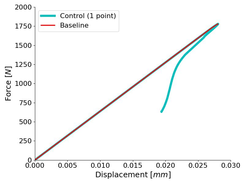
Figure 4. The control-based method is able of following the load-displacement curve even with decreasing displacement
The load-displacement curves of the DENT model using the COD-control technique and the baseline model are plotted in Figure 4. We can see that the baseline model becomes unstable after the peak load and the job aborts (red line), whereas the controlled FE model is able to capture the load drop with snap-back plus all the crack propagation process that takes place after the peak load (cyan line).
Yes! We did it! We have been able to capture this cracking process including a very sharp snap-back!
4. Example 2: Make it more stable
Stability of the previous model falls upon the relative displacement of just two nodes (\(C_1\) and \(C_2\)), which may be risky after a long crack propagation. To tackle this limitation, we can define the control variable as the summation of all the CODs of all the pairs of nodes along the crack.
$$f_y^{DN} = u_y^{C_1} – u_y^{C_2}$$
$$f_y^{DN} = u_y^{C_3} – u_y^{C_4}$$
$$f_y^{DN} = u_y^{C_5} – u_y^{C_6}$$
$$…$$
It should be noted that each of these equations adds up to the total force on DN, or what is the same, the total force on DN is equal to the summation of all the CODs.
The input file corresponding to this example is ‘DENT_controlmulti.inp‘
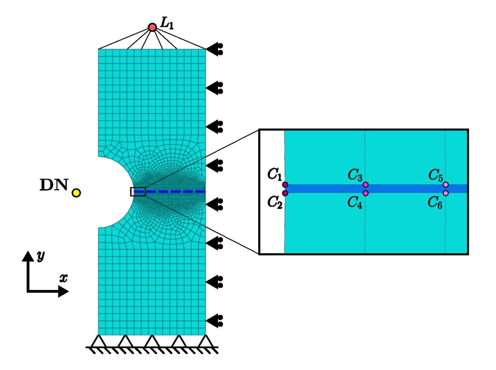
Figure 5. Pairs of nodes that define locally the COD along the crack path.
4.1 - Implementation in Abaqus
The main difference in this case is that we require as many elements as pairs of nodes (local CODs) we want to consider along the crack path.
- inp
					** Create elements for eq. 1 (connectivity)
*Element, type=U101, elset=auxiliary
** label, node_C1, node_C2, node_DN
 1000001,      13,      15,   5269
 1000002,     330,     439,   5269
 1000003,     331,     440,   5269
 ...
 1000101,     429,     538,   5269
 1000102,      14,      16,   5269
**
- Lines 4-9. One user element is created for every pair of nodes along the crack path to impose eq. (1). A total of 102 elements are defined in this model.
- The definition of the elements U101 and U102 does not change.
It must be noted that the force applied on DN represents the summation of all the CODs, that’s why in this case the value applied is much higher:
- inp
					** Control variable: Force applied on director node controls the
** cumulative crack opening (!)
*Cload
DN, 2, 0.99
4.2 - Results
In this case, the simulation can go even further than before which evidences the superior stability using multiple CODs along the crack path.
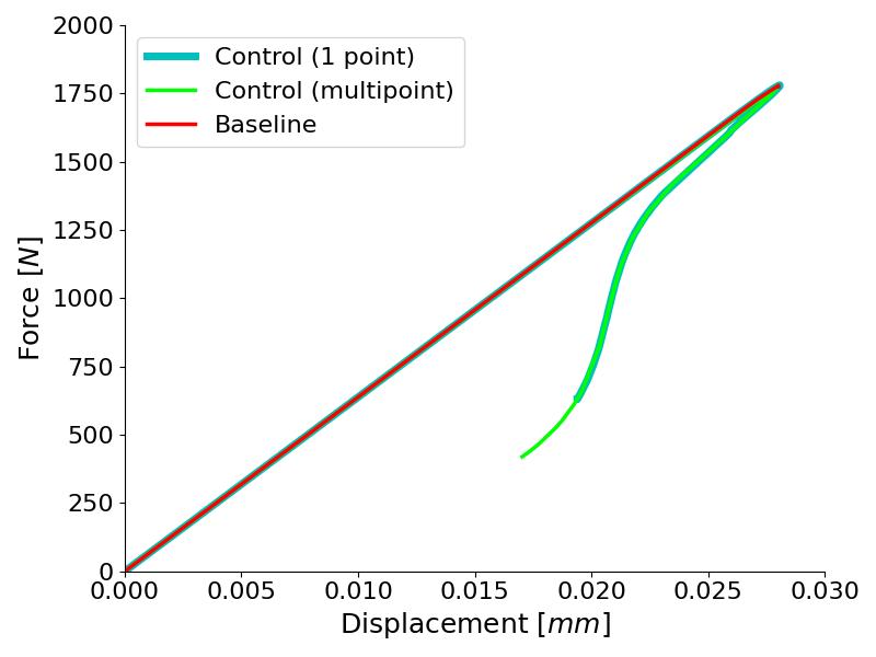
Figure 6. Comparison of single-point and multi-point control methods
Quick tip!
In the odb visualization, every user element is represented by a white cross. Sometimes this may be annoying. To hide these white crosses from the visualization go to:
Odb display options → Entity display → Disable “Show point elements“
Let’s see another case where this control technique was crucial in one of my research topics.
5. Example 3: Advanced buckling model
A few years back, after completing my Phd, I was still working in Computational Micromechanics models to understand how unidirectional fiber-reinforced plies fail under longitudinal compression. I developed a model made of a single carbon fiber surrounded by polymer matrix following a wavy trajectory (sine curve) and applied a longitudinal compressive load.
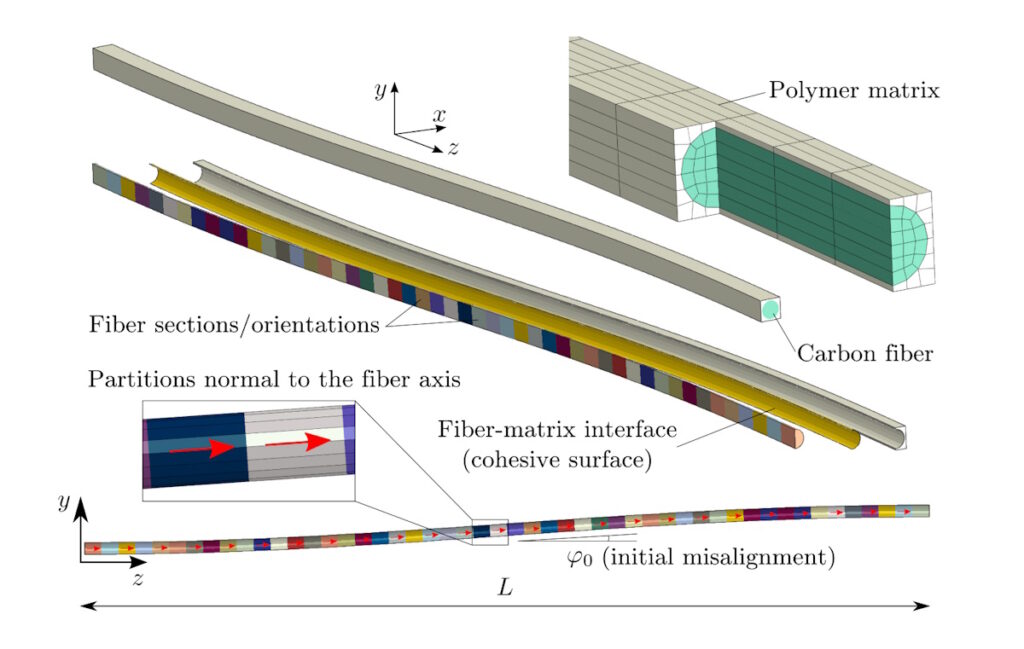
Figure 7. Exploded cut view and side view of the single-fiber model to study longitudinal compression [NASA/TP–2018–220105]
Guess what… Yes, it looks like a buckling problem. Everything is linear and elastic until the peak load, after which there is a lot of snap-back. Solving this simulation was a big problem because I wanted to predict the compressive strength and also the residual stress after collapse. By the way, the failure mechanism triggered after peak load is called fiber kinking.
I started using implicit dynamic steps, which worked reasonably well. But eventually, I discovered the control technique, I put it into practice and it was outstanding.
The input file corresponding to this example is ‘kinking_control.inp‘
Let me show you how to apply the control technique to this buckling problem.
5.1 - The control variable
The first task is to identify which is the control variable, the main condition to fulfil is that it must increase monotonically along the simulation.
After some inspection and experience testing the model, I found that the transverse displacement of the front end of the model worked well (\(u_y^{RP}\)). Therefor, the first equation boils down to \(f_y^{DN} = u_y^{RP}\). Note that RP is a reference point coupled to the front face of the model.
On the other hand, the compressive load is applied through RP using the degree of freedom 3 (\(u_z^{RP}\)). Therefor, equation 2 is \(f_z^{RP} = -u_y^{DN}\) (negative because of the compressive loading).
Writing both conditions in matrix form considering 2 nodes and 2 degrees of freedom (y and z), we end up with:
$$\underbrace{\begin{bmatrix}
0 & 0 & 0 & 0 \\
0 & 0 & -1 & 0 \\
1 & 0 & 0 & 0 \\
0 & 0 & 0 & 0
\end{bmatrix}}_{K}
\begin{Bmatrix}
u_y^{RP} \\
u_z^{RP} \\
u_y^{DN} \\
u_z^{DN}
\end{Bmatrix}
=
\begin{Bmatrix}
f_y^{RP} \\
f_z^{RP} \\
f_y^{DN} \\
f_z^{DN}
\end{Bmatrix}$$
5.2 - Implementation in Abaqus
Following the same reasoning shown in previous examples, the implementation only requires one custom user element made of 2 nodes and 2 degrees of freedom per node:
- inp
					** RP - Loading and control
*NODE, NSET=RP
 2000000, 0., 0., 500.
**
** DN - Director node for control algorithm
*Node, nset=DN
 2000001, 0., 0., 510.
**
** Definition of first auxiliary element RP (y,z) - DN (y,z)
** Degrees of freedom used by this user element (y & z)
*User element, nodes=2, type=U100, linear, unsymm
 2, 3
**
*Matrix, type=stiffness
1e-12,    0.,    0.,    0.
    0, 1e-12,    1.,    0.
    0,   -1., 1e-12,    0.
    0,    0.,    0., 1e-12
**
** Create the element (connectivity)
*Element, type=U100, elset=aux
** label, node_RP, node_DN
  200001, 2000000, 2000001
**
*Uel property, elset=aux
- Lines 2-3 & 6-7. First we create the nodes RP and DN. The position of these auxiliary nodes in the model is irrelevant.
- Lines 11-12. The custom user element (U100) is made of 2 nodes and requires 2 dof \((u_y, u_z)\).
- Lines 14-18. The stiffness matrix \(K\) is 4-by-4, defined column-wise.
- Lines 21-23. The user element label is 200001, connecting RP and DN.
5.3 - Results
The main results from the history output are:
- The longitudinal displacement (U3) of RP.
- The force applied through RP which is the transverse displacement (U2) of DN. Negative because it’s compression.
Load-displacement curves are summarized in Figure 8. The reference model solved using a static step under conventional displacement control is able to find a solution by skipping the snap-back section (red line), but the plastic deformation pattern is affected and the residual stress predicted does not match the exact solution achieved by the control technique presented (cyan line). In addition, the novel method captures the full load-displacement curve with snap-back. Hence, illustrating progressively how fiber kinking develops in detail.
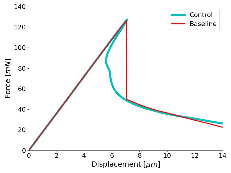
Figure 8. Longitudinal compression curves in the fiber kinking model
This control technique will let you stabilize buckling problems, you only need to identify and track the right control variable.
6. Conclusions
Convergence is one of the main obstacles that FE analysts have to face more often.
In this blog post, we have shown a control methodology based on tracking a variable that increases monotonically along the simulation like the COD in fracture problems.
Another well-known algorithm built-in Abaqus to address snap-back problems is the modified Riks method. Riks is capable of capturing smooth snap-back cases, but it may not converge if the load-displacement curve turns very sharply.
The main advantage of the control algorithm presented here is the stability. This method is able to solve problems with acute snap-back features. However, it introduces an additional cost in the solver as it breaks the symmetry of the global stiffness matrix of the problem which may increase the computational cost of the simulation.
So, if you need to stabilize your FE model or you are concerned with snap-back, go ahead and give it a try!
And if you are looking forward to implement your own user elements (UEL) to enable custom FE simulations in Abaqus, don’t miss the course “User Subroutines in Abaqus”. You’ll gain expertise in Fortran subroutines, a powerful tool that’s both highly in demand and surprisingly rare among Abaqus users. This unique knowledge will give you the edge you’re looking for. Don’t miss the opportunity to set yourself apart! Check it out!
I hope that you find these tips useful!
