SIMULATION OF COMPOSITE MATERIALS WITH ABAQUS
Learn the most relevant modeling techniques for composites understanding HOW and WHY

Discover the most valuable and efficient numerical strategies to get high-quality simulations of composite materials

Understand all the concepts behind the FE models: multiscale modeling, cohesive zone models, periodic boundary conditions, residual stresses, damage modeling…

Save lots of time automating your numerical models thanks to Python scripts in Abaqus

Learn how to fix your simulation if it does not converge, even in the presence of damage and other nonlinearities

Learn how to interpret the results of your numerical models and a lot more tips and recommendations to obtain stunning and meaningful visualizations
My name is Miguel Herráez, I am an industrial engineer and Phd in Materials Science.
My first contact with Composite Materials was at the end of my BSc in Mechanical Engineering, performing my final project in the US (West Virginia University).
Thanks to my Advisor (Prof. Ever Barbero), I started to get more and more involved in that field. At that moment, I did not know that it was just the beginning of my scientific career.
I have been studying, testing and developing Finite Element (FE) simulations since 2013, when I started my Phd on numerical modeling of fiber-reinforced composites. I still remember the first years in which I had to learn very little by little about this topic on my own.
For that reason, I have finally prepared this course with which I want you to learn the numerical strategies for the simulation of composite materials.
You will learn in some hours all what I have learnt in almost 10 years!

Visiting researcher
Post-doctoral researcher
Industrial and scientific projects
BSc final project
Research assistant
Lecturer
Phd in Mechanics of Materials
BSc in Industrial Engineering
Structure of the course
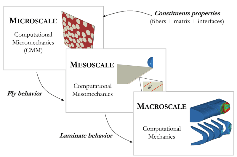
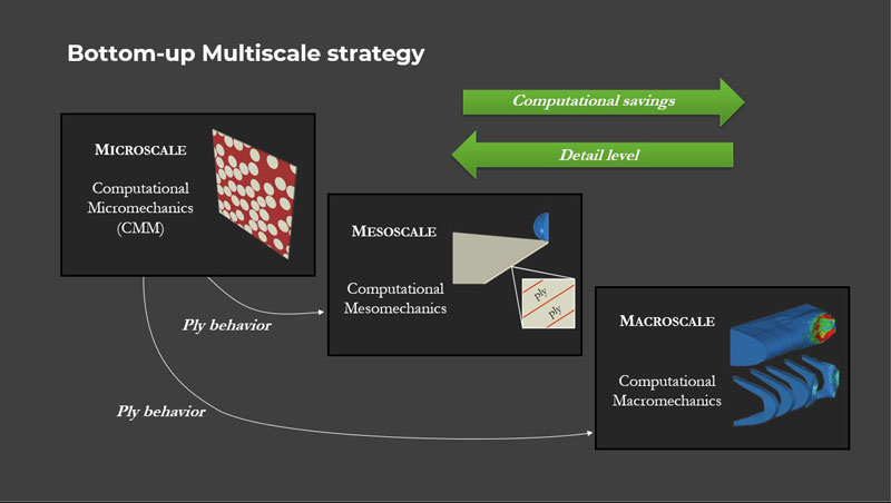
- The course follows the Bottom-up Multiscale strategy and is organized into 3 main chapters: Comp. Micromechanics, Comp. Mesomechanics and Comp. Macromechanics.
- Computational Micromechanics is the mainstay to understand and model the deformation mechanisms of composite materials starting at the constituents scale.
- Whereas Mesomechanics is the perfect framework to simulate real-scale components (mm to cm), and at the same time to reproduce all the failure mechanisms of composite plies and laminates.
- Computational Macromechanics combines a set of modeling assumptions that make possible the numerical analysis of large components and composite structures (scale of meters).
- The course is made of more than 26 hours organized into more than 170 videos and a lot of additional resources: Python scripts, exercises, scientific papers and technical reports, links to specific sections of the documentation…
- The course compiles all what I have learnt about the simulation of composite materials along almost 10 years of thousands of trial-and-errors, extensive literature reviews and many discussions with colleagues in this field.
- Every 2 hours of the course, you will save 1 full year of testing on your own: aborted simulations, periodic boundary conditions not working, meshing problems, issues with cohesive elements, interpretation mistakes, visualization improvements…

ACCESS FOR LIFE
Access this course forever. Watch the videos and review the lessons anytime, at your own pace

CERTIFICATE
After finishing the course you will get your certificate of completion

RESOURCES
You will get all the scripts, programs, examples and quizzes of the course

QUESTIONS
I will solve all your questions throughout the course
Check the contents of the course:
Simulation of Composite Materials with Abaqus
The course is made of 5 chapters, containing +26 hours of video, organized into +170 lessons, +60 Python scripts, +40 technical papers and references
CLICK on the chapters below to check out the contents
1
Introduction to composites
2
Computational Micromechanics
3
Computational Mesomechanics
4
Computational Macromechanics
5
Conclusions and challenges
- 1.1 – 🎬 Introduction to composite materials
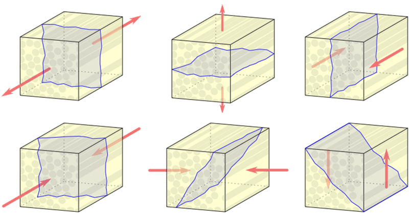
- 2.1 – 🎬 The Bottom-up Multiscale strategy
- 2.2 – Structure of the course
- 1.1 – Introduction to composite materials
- 1.1.1 – 🎬 Introduction to CMM
- 1.2 – Numerical strategies for CMM
- 1.2.1 – 🎬 CMM: Periodic RVEs
- 1.3 – Structure of the chapter
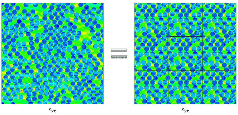
- 2.1 – Development of a unit cell model
- 2.1.1 – 🎬 Presentation of the model
- 2.1.2 – 🎬 Creation of the part
- 2.1.3 – 🎬 Meshing the part
- 2.1.4 – 🎬 Assembly and boundary conditions
- 2.1.5 – 🎬 Job and first results
- 2.2 – Periodic boundary conditions (PBC)
- 2.2.1 – 🎬 Introduction to PBC
- 2.2.2 – 🎬 Creation of a 2D unit cell
- 2.2.3 – 🎬 Definition of equations in Abaqus
- 2.2.4 – 🎬 Script to generate PBC in 2D (1/2)
- 2.2.5 – 🎬 Script to generate PBC in 2D (2/2)
- 2.2.6 – 🎬 Including PBC in the model
- 2.2.7 – 🎬 Definition of PBC in 3D
- 2.2.8 – 🎬 Computing the Poisson ratios using master nodes
- 2.3 – Automatic generation of the FE model using a Python script
- 2.3.1 – 🎬 Script of the unit cell model (1/4)
- 2.3.2 – 🎬 Script of the unit cell model (2/4)
- 2.3.3 – 🎬 Script of the unit cell model (3/4)
- 2.3.4 – 🎬 Script of the unit cell model (4/4)
- 2.3.5 – 🎬 Script of the RVE model (1/3)
- 2.3.6 – 🎬 Script of the RVE model (2/3)
- 2.3.7 – 🎬 Script of the RVE model (3/3)
- 2.4 – Algorithm to generate random microstructures
- 2.4.1 – 🎬 Theory: Random Sequential Absorption algorithm
- 2.4.2 – 🎬 Implementation in a script (1/2)
- 2.4.3 – 🎬 Implementation in a script (2/2)
- 2.4.4 – 🎬 Visualization of the microstructures
- 2.4.5 – 🎬 Jamming limit and tolerance distance
- 2.4.6 – 🎬 Some visualization tips
- 2.4.7 – 🎬 Transformation of the RSA algorithm into a function
- 2.4.8 – 🎬 Integration of RSA in the FEA worflow
- 2.4.9 – 🎬 Advanced scripting: Exceptions
- 2.5 – Computing the elastic properties of the UD ply
- 2.5.1 – 🎬 How to compute the elastic properties
- 2.5.2 – 🎬 Computing the elastic properties in Abaqus
- 2.5.3 – 🎬 Definition of the normal loading cases
- 2.5.4 – 🎬 Definition of the shear loading cases
- 2.5.5 – 🎬 Automating the postprocess (1/2)
- 2.5.6 – 🎬 Automating the postprocess (2/2)
- 2.5.7 – 🎬 Analysis of the results: Elastic properties
- 2.5.8 – 🎬 Simulation of thermal expansion
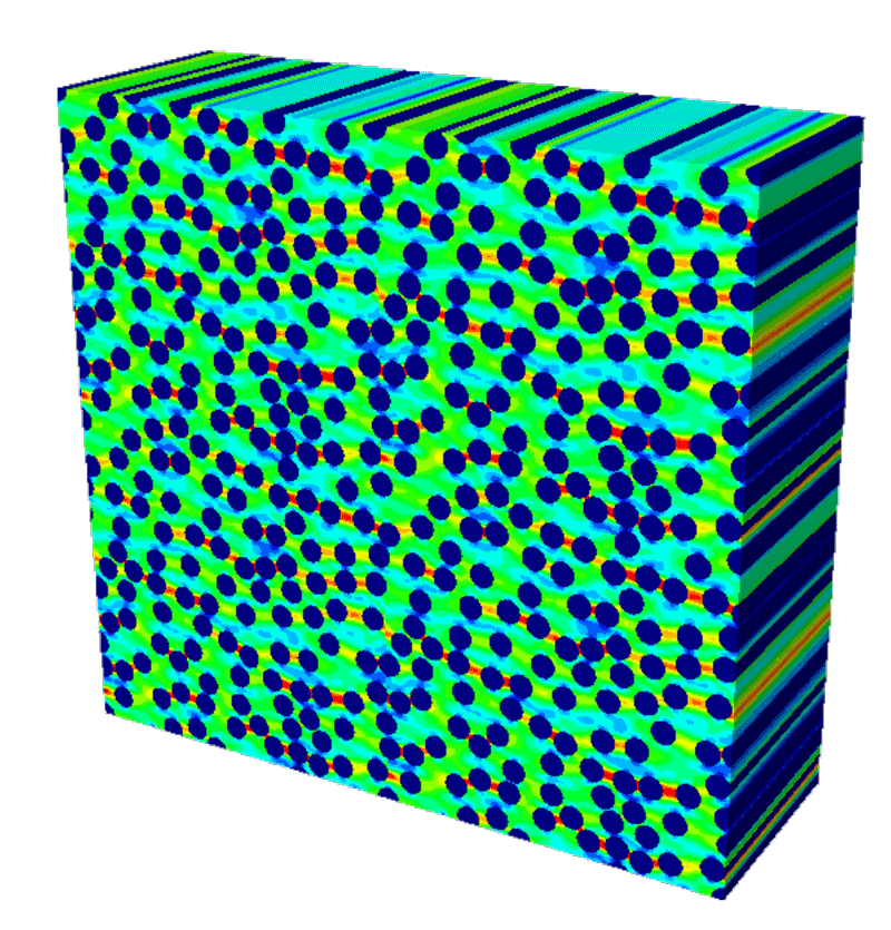
- 3.1 – Limitations of the periodic RVE models
- 3.1.1 – 🎬 Periodic RVEs have limits
- 3.2 – Inelastic deformation of the constituents
- 3.2.1 – 🎬 Micromechanical inelastic deformation mechanisms
- 3.2.2 – 🎬 Matrix: Plastic deformation
- 3.2.3 – 🎬 Interface: Cohesive Zone Model
- 3.3 – Modifications in the RVE model
- 3.3.1 – 🎬 Preparation of a script to generate the new model
- 3.3.2 – 🎬 Insertion of cohesive elements along the interfaces (1/3)
- 3.3.3 – 🎬 Insertion of cohesive elements along the interfaces (2/3)
- 3.3.4 – 🎬 Insertion of cohesive elements along the interfaces (3/3)
- 3.3.5 – 🎬 Convergence issues and final touches
- 3.4 – Loading cases
- 3.4.1 – 🎬 Transverse tension
- 3.4.2 – 🎬 Review of transverse tension case
- 3.4.3 – 🎬 Transverse compression
- 3.4.4 – 🎬 Longitudinal shear
- 3.4.5 – 🎬 Transverse shear
- 3.4.6 – 🎬 Residual thermal stresses
- 3.5 – Solving common problems
- 3.5.1 – 🎬 Issue #1: PBC not working
- 3.5.2 – 🎬 Issue #2: Instance not meshed
- 3.5.3 – 🎬 Issue #3: Invalid mesh
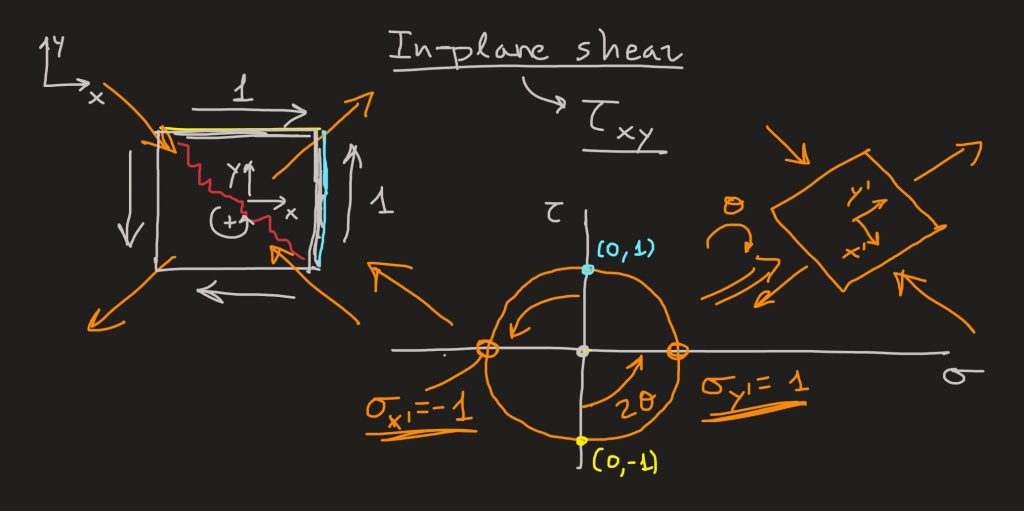
- 4.1 – Computational Micromechanics is more than RVEs
- 4.1.1 – 🎬 Alternatives to periodic RVEs
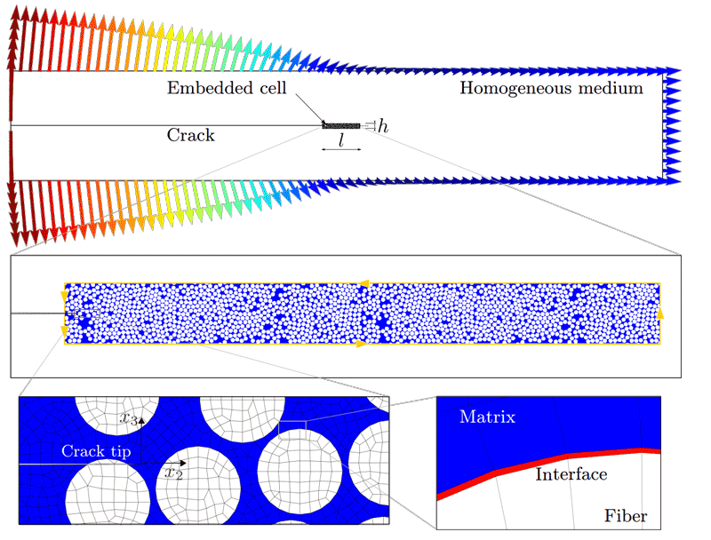
- 1.1 – 🎬 Introduction to Computational Mesomechanics
- 1.2 – 🎬 Naming convention of laminate stacking sequences (LSS)
- 1.3 – Structure of this chapter
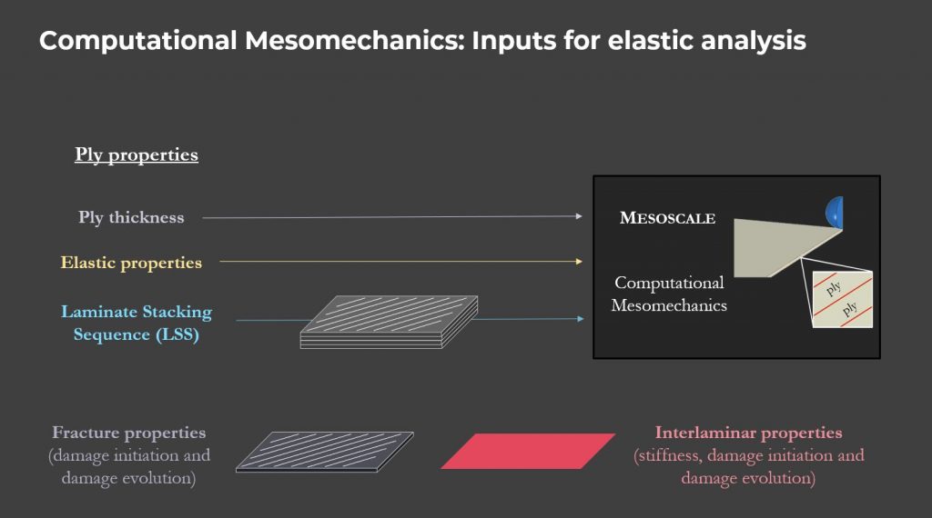
- 2.1 – Development of the elastic FE model of the pinned joint
- 2.1.1 – 🎬 Presentation of the model
- 2.1.2 – 🎬 Pinned joint: Part
- 2.1.3 – 🎬 Pinned joint: Mesh
- 2.1.4 – 🎬 Pinned joint: Material
- 2.1.5 – 🎬 Pinned joint: Assembly
- 2.1.6 – 🎬 Pinned joint: Contact
- 2.1.7 – 🎬 Pinned joint: Rigid pin
- 2.1.8 – 🎬 Pinned joint: Boundary conditions
- 2.1.9 – 🎬 Pinned joint: Results
- 2.2 – Automating the generation of the FE model using Python script
- 2.2.1 – 🎬 Python script of the pinned joint: Sketch and part
- 2.2.2 – 🎬 Python script of the pinned joint: Sets and partitions of the plies
- 2.2.3 – 🎬 Python script of the pinned joint: More partitions
- 2.2.4 – 🎬 Python script of the pinned joint: Mesh, material and sections
- 2.2.5 – 🎬 Python script of the pinned joint: From assembly to job
- 2.2.6 – 🎬 Python script of the pinned joint: Final
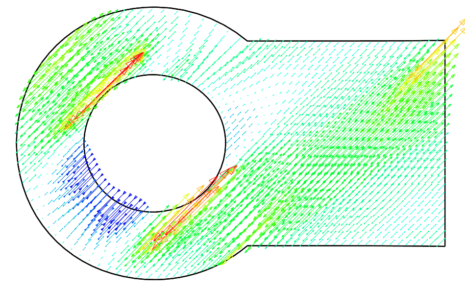
- 3.1 – Introduction to failure criteria of materials
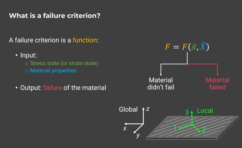
- 3.1.1 – 🎬 Fundamentals of failure criteria of materials
- 3.1.2 – 🎬 Failure criteria of composite materials
- 3.2 – Failure criteria of composites in Abaqus
- 3.2.1 – 🎬 Modification of the model: Hashin material properties
- 3.2.2 – 🎬 Modification of the model: Mesh, section and output
- 3.2.3 – 🎬 Including the Hashin criterion in the script
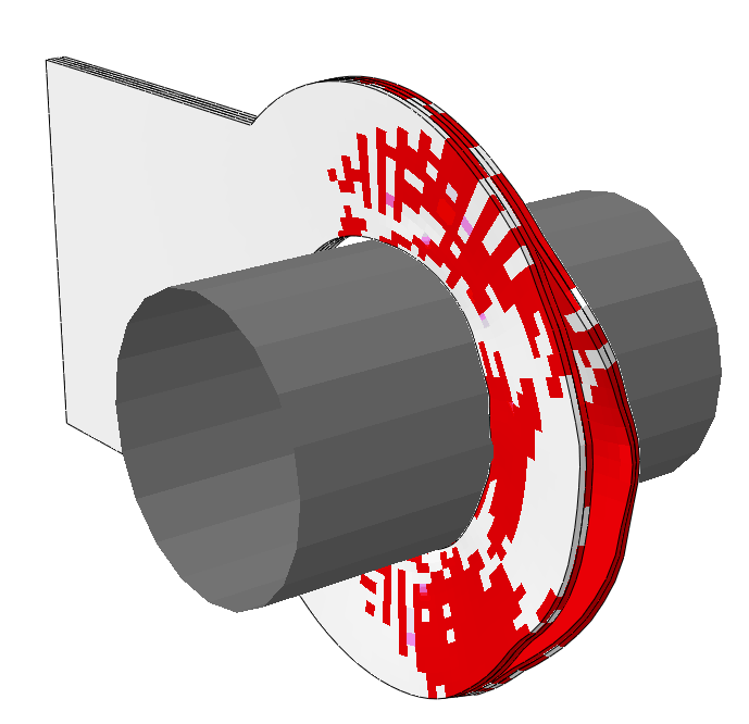
- 4.1 – Introduction to damage of composite materials at the mesoscale
- 4.1.1 – 🎬 Modeling damage in mesomechanical models
- 4.2 – Modeling intralaminar damage
- 4.2.1 – 🎬 Damage evolution parameters in Abaqus
- 4.2.2 – 🎬 Damage and loss of convergence
- 4.2.3 – 🎬 Stabilizing the model through viscous dissipation
- 4.2.4 – 🎬 Hashin damage variables
- 4.2.5 – 🎬 Hashin damage: Python script
- 4.2.6 – 🎬 Understanding damage evolution in CDM
- 4.2.7 – 🎬 Element size dependence in CDM
- 4.3 – Modeling interlaminar damage I (cohesive elements)
- 4.3.1 – 🎬 Introduction to interlaminar damage
- 4.3.2 – 🎬 Interlaminar properties
- 4.3.3 – 🎬 Making the partitions for the cohesive elements
- 4.3.4 – 🎬 Finishing the model with cohesive elements
- 4.3.5 – 🎬 Results and damage initiation criterion
- 4.4 – Convergence, solvers and steps
- 4.4.1 – 🎬 Implicit dynamic step
- 4.4.2 – 🎬 Implicit vs. Explicit
- 4.4.3 – 🎬 Explicit step: Abaqus/CAE
- 4.4.4 – 🎬 Explicit step: Script
- 4.4.5 – 🎬 Stable time increment
- 4.5 – Fracture Process Zone (FPZ)
- 4.5.1 – 🎬 Definition of fracture process zone
- 4.5.2 – 🎬 How to use a coarse mesh along the FPZ
- 4.5.3 – 🎬 Implications and limitations tuning the FPZ
- 4.5.4 – 🎬 Results: delamination
- 4.6 – Modeling interlaminar damage II (cohesive surfaces)
- 4.6.1 – 🎬 Introduction to cohesive surfaces modeling
- 4.6.2 – 🎬 Definition of cohesive contact in Abaqus/Explicit
- 4.6.3 – 🎬 Scripting the cohesive contacts
- 4.6.4 – 🎬 Cohesive elements vs. Cohesive surfaces
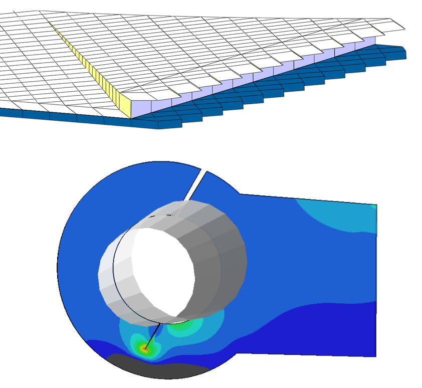
- 5.1 – 🎬 Summary
- 5.2 – 🎬 State of the art: Techniques and theories
- 1.1 – 🎬 Introduction to Computational Macromechanics
- 1.2 – Structure of this chapter
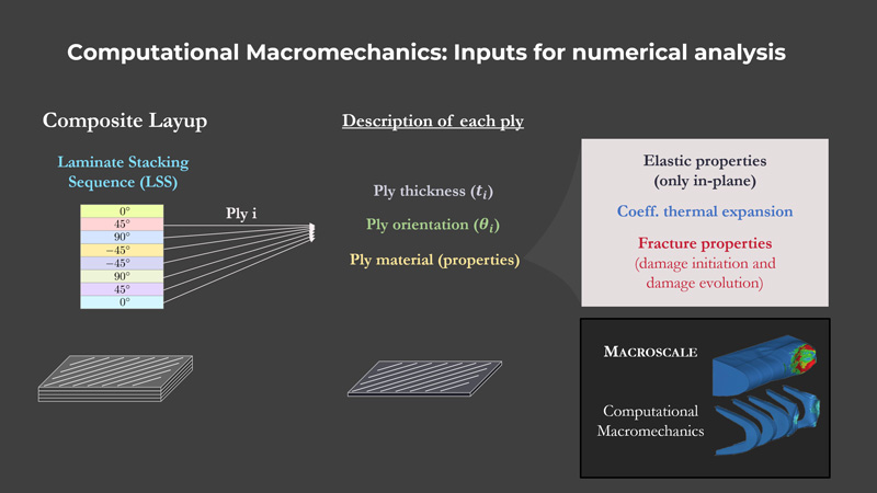
- 2.1 – Development and analysis of equivalent models with different element types
- 2.1.1 – 🎬 Presentation of the model
- 2.1.2 – 🎬 Case 1: C3D8R x 1 (preprocess)
- 2.1.3 – 🎬 Case 1: C3D8R x 1 (results)
- 2.1.4 – 🎬 Case 2: C3D8R x 5
- 2.1.5 – 🎬 Case 2: C3D8R x 5 (verification)
- 2.1.6 – 🎬 Case 3: C3D8 x 5
- 2.1.7 – 🎬 Case 4: SC8R
- 2.1.8 – 🎬 Case 5: S4R
- 2.1.9 – 🎬 Visualization of results in shell elements
- 2.1.10 – 🎬 Summary and one more case
- 2.2 – Analytical solution of the doubly-clamped beam
- 2.2.1 – Solving the problem
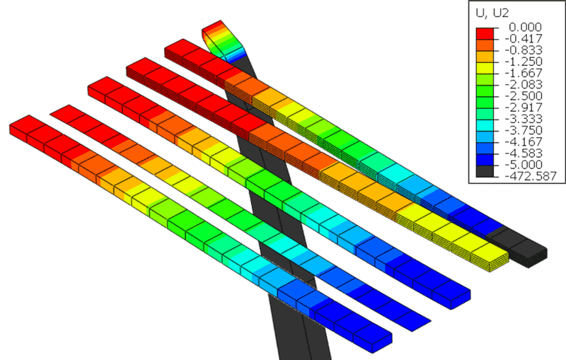
- 3.1 – Definition of Composite Layups in Abaqus
- 3.1.1 – 🎬 Introduction to Composite Layups in Abaqus
- 3.1.2 – 🎬 Example 1: Unidirectional laminate (preprocess)
- 3.1.3 – 🎬 Example 1: Unidirectional laminates (analysis)
- 3.1.4 – 🎬 Example 2: Cross-ply laminate
- 3.1.5 – 🎬 Example 3: Cross-ply hybrid laminate
- 3.1.6 – 🎬 Example 4: Non-symmetric cross-ply
- 3.1.7 – 🎬 Example 5: Anti-symmetric balanced laminate
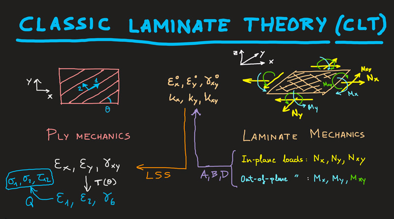
- 3.2 – Classic Laminate Theory (CLT)
- 3.2.1 – 🎬 Introduction to CLT
- 3.2.2 – 🎬 Ply Mechanics
- 3.2.3 – 🎬 Laminate Mechanics
- 3.2.4 – 🎬 Laminate matrices under in-plane loading
- 3.2.5 – 🎬 Laminate matrices under out-of-plane loading
- 3.2.6 – 🎬 Symmetric laminates and some remarks
- 3.3 – Verification of numerical models
- 3.3.1 – 🎬 Putting CLT into practice
- 3.3.2 – 🎬 Analyses of symmetric laminates (ex. 1, 2 & 3)
- 3.3.3 – 🎬 Analysis of non-symmetric cross-ply (ex 4)
- 3.3.4 – 🎬 Analysis of anti-symmetric balanced laminate (ex 5)
- 3.3.5 – 🎬 How to get the A, B, D matrices in Abaqus
- 3.4 – Effective laminate moduli
- 3.4.1 – 🎬 In-plane laminate moduli
- 3.4.2 – 🎬 Out-of-plane laminate moduli
- 4.1 – Introduction and analysis of the initial design
- 4.1.1 – 🎬 Pressurized vessel: Introduction
- 4.1.2 – 🎬 Pressurized vessel: Part and mesh
- 4.1.3 – 🎬 Pressurized vessel: Material and section
- 4.1.4 – 🎬 Pressurized vessel: BCs and job
- 4.1.5 – 🎬 Pressurized vessel: Preliminary analysis
- 4.1.6 – 🎬 Pressurized vessel: Cross-ply laminate
- 4.1.7 – 🎬 Custom field output
- 4.2 – Optimization of the laminate
- 4.2.1 – 🎬 Optimality vs. Versatility
- 4.2.2 – 🎬 Design of a balanced laminate
- 4.2.3 – 🎬 Modification of the original laminate
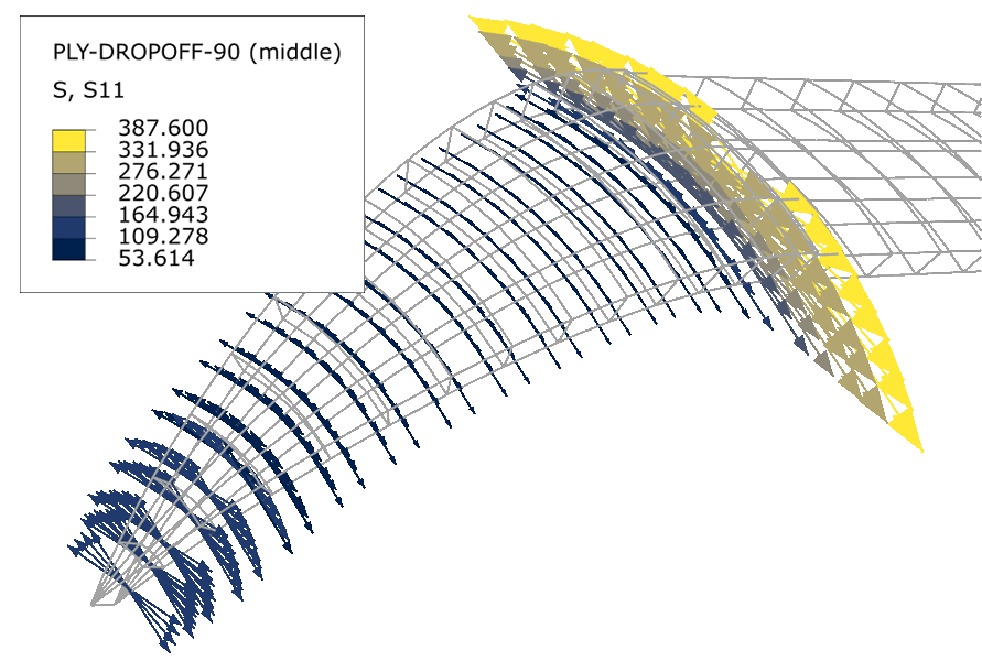
- 4.2.4 – 🎬 Further optimization: Ply drop-off
- 4.3 – New ply failure criteria: LaRC05
- 4.3.1 – 🎬 How are jobs run by Abaqus?
- 4.3.2 – 🎬 LaRC05: Introduction
- 4.3.3 – 🎬 LaRC05: Parameters
- 4.3.4 – 🎬 Including the LaRC05 criterion in the input file
- 4.3.5 – 🎬 How to run a model from the input file: 2 methods
- 4.4 – Thermal residual stresses
- 4.4.1 – 🎬 Introduction to thermal stress
- 4.4.2 – 🎬 Thermal residual stresses in composite laminates
- 4.4.3 – 🎬 Thermal stresses in Abaqus
- 4.5 – Sandwich laminate for cryogenic applications I
- 4.5.1 – 🎬 Design proposal
- 4.5.2 – 🎬 Sandwich laminate: Part
- 4.5.3 – 🎬 Sandwich laminate: Mesh
- 4.5.4 – 🎬 Sandwich laminate: Materials and sections
- 4.5.5 – 🎬 Sandwich laminate: Full model
- 4.5.6 – 🎬 Sandwich laminate: Results (only pressure)
- 4.6 – Sandwich laminate for cryogenic applications II
- 4.6.1 – 🎬 Modeling the cooling down to cryogenic conditions
- 4.6.2 – 🎬 Analysis of the final results
- 4.6.3 – 🎬 Final comments
- 5.1 – 🎬 Conclusions
- 5.2 – 🎬 Macromechanics or Mesomechanics
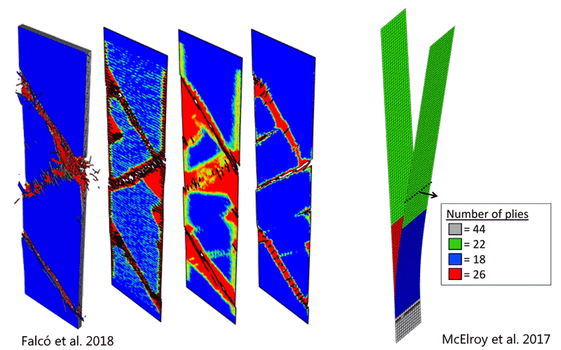
- 1.1 – 🎬 State of the art across the scales
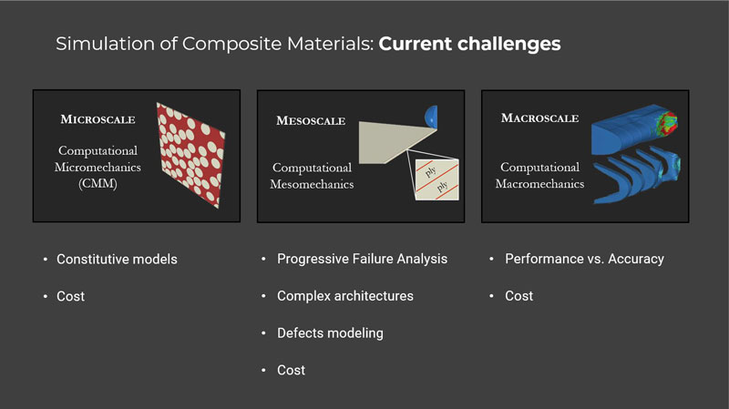
- 2.1 – 🎬 Current challenges and opportunities
The course is based on these three pillars:
WHY – HOW – WHAT
- Why do we design the model in such or such way? Learn to analyze and design finite element models based on experimental observations supported by theoretical explanations.
- How do we implement this design into an FE model? Learn step-by-step how to develop the FE models in Abaqus from scratch. In all cases, we will also learn how to generate and customize a Python script to automate and parameterize all the workflow.
- What is the interpretation of the results? Learn the meaning of each result and how to obtain stunning visualizations. You will get the basis to interpret the results of any other finite element simulation.
You will not only learn to design, build and solve the models covered during the course, but also you will be ready to develop a thousand more types of models!
I have invested a lot preparing this course and I am really proud of the result. I strongly believe that it is going to be super useful for you and a huge time-saver.
What my students think of the course


In the course you will find…
- +26 h of recorded videos
- +170 video lessons
- +60 Python scripts
- +40 papers and references
- Fully compatible with Abaqus Learning Edition
- Access for life to the course
- Access to all new contents and updates
- Personal support
- Certificate of completion
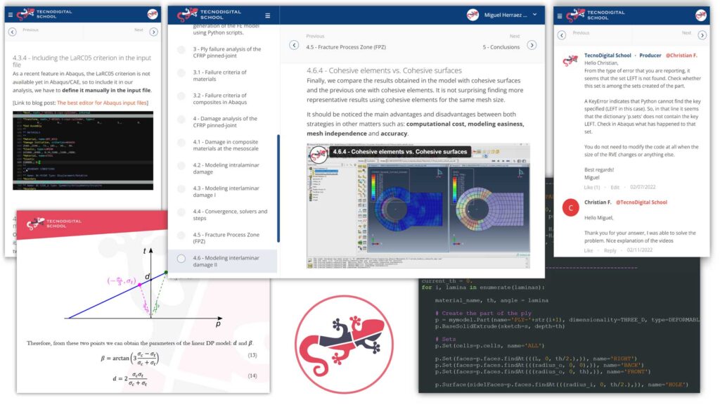
Theoretical explanations
+
Practical cases

The course provides an unconditional money-back guarantee.
Join without any commitment. If you are not satisfied, we will refund all your money within the first 15 days.
Send an email to contact@tecnodigitalschool.com, and request your refund. The only condition is that you shall not have watched more than 20% of the course.
Wanna take a look inside?

SIMULATION OF COMPOSITE MATERIALS WITH ABAQUS
5 blocks of contents
+170 lessons
+26 h of recorded videos
+60 Python scripts
+40 papers and references
Fully compatible with Abaqus Learning Edition


Do you have any questions about the course Simulation of Composite Materials with Abaqus?
This course is made of +170 video lessons (5 to 20 minutes long) which are organized into 5 chapters of contents as detailed above.
All the scripts developed and lots of additional resources are given next to each of the videos, as well as more documentation and references to go deeper into all the details
There are thousands of resources on the internet, documentation, tutorials, videos on Youtube… The problem is that you will struggle bringing together all these bits and bytes of information.
Not to mention, this will take you a huge amount of time.
That's why in this course I have collected my experience, almost 12 years working on simulation of composites almost daily, and I know which are the hardest concepts and most common difficulties.
Anyways, if you don’t take this course, I recommend you to count on good learning examples, to study the official documentation of Abaqus and work with a person with a huge expertise in this field to help you clarify the toughest concepts.
Otherwise, you will enter this group of professionals who are able to design and implement simulations of composite materials and understand the what-how-why of their simulations with my support. It is your decision.
This course will make you stand out of the crowd when applying to job positions in the expanding composites market.