Abaqus is one of the best simulation softwares available nowadays. However, CAD features within the Part module are limited and may not be sufficient to generate complex 3D geometry. Or maybe, we already have external CAD geometry in standard format files (stl, iges, stp…) that we need to use straightforward.
Abaqus supports importing many of these CAD formats and permits its inclusion in finite element (FE) analysis.
We will see an example in which we have two STP files that are imported into Abaqus and manipulated to mesh and incorporate them in a numerical simulation.
1. The FE model
The FE model developed will be the impact of a hammer onto a shield. And yes, it’s Thor’s hammer (Mjolnir) impacting against the only object that can withstand such devastating power: Captain America’s shield!
All the assets and the script required to generate this model in Abaqus can be downloaded here. You will find two folders inside: one to create the fully detailed model (full_version) and another one with not as many details that is affordable through the Abaqus student edition (student_edition) to create a model with less than 1000 nodes.
Note: some Abaqus student editions have issues importing STP files, so the same CAD parts are provided in Standard ACIS Text format (SAT) as well.
2. Importing geometry in Abaqus
2.1 Importing the hammer
The hammer was imported into Abaqus by going to: File → Import → Part… And selecting the file with the geometry of the hammer (hammer.stp or hammer.sat). In the dialog that appears we leave the options by default, making sure that the part created will be 3D and deformable.
We can automate the process of importing geometry through a Python script, in this way the whole generation of the model is parameterized with the following lines:
- Python
					# Usual imports to run Abaqus commands
from abaqus import *
from abaqusConstants import *
from caeModules import *

# New model
Mdb()

# Import stp file
stp = mdb.openStep('hammer.stp')

# Create part from stp geometry
p = mdb.models['Model-1'].PartFromGeometryFile(
                        name='hammer',
                        geometryFile=stp,
                        dimensionality=THREE_D,
                        type=DEFORMABLE_BODY)

#----------------------------------------------
- Lines 1 to 4: Standard imports to run Abaqus commands
- Line 7: Create a new empty model
- Line 10: Import the STP file
- Lines 13 to 17: Create a new part from the imported STP file
After making some partitions, the hammer can be properly meshed using solid hexaedral elements. Then, elastic properties and density are asigned and the part is ready to be instantiated in the assembly!

2.2 Importing the shield
The shield is imported following the same procedure:
File → Import → Part…: shield.stp or shield.sat
When importing the shield, a message will pop up with a warning about “imprecise geometry”. Don’t panic, there are some tiny edges that will put us in trouble when meshing this part. We will fix it by selecting “Repair Small Edges” in the Part module.


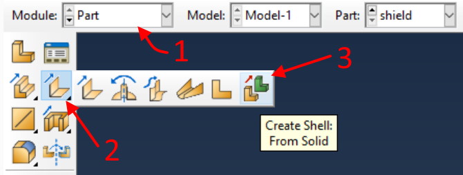
The shield is represented as a volume, it is made of cells like the hammer (it is thick). However, it is not very efficient to model this sort of structure using solid elements. Instead, for the simulation we would like to keep only the front faces of the shield and mesh them with shell elements. To do this, we can get rid of the cells of the model by selecting “Create Shell: From Solid” in the Part module, so only the outer shell remains (external faces).
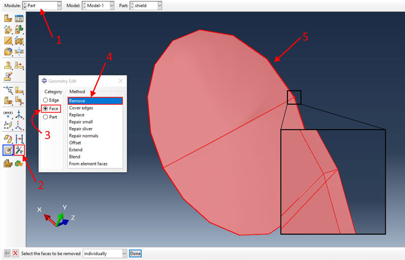
Then, we can delete unnecessary faces for the simulation, i.e. rear faces and the lid around the shield. In the Part module, go to: Geometry Edit → Face → Remove and select those faces.
The operations made so far on the shield are automated with the following script:
- Python
					# Usual imports to run Abaqus commands
from abaqus import *
from abaqusConstants import *
from caeModules import *

# Shield part
step = mdb.openStep('shield.stp')
ps = mdb.models['Model 1'].PartFromGeometryFile(name='shield', geometryFile=step,
          combine=False, dimensionality=THREE_D, type=DEFORMABLE_BODY)

# Merge vertices that are too close
ps.RepairSmallEdges(edgeList=ps.edges[:], toleranceChecks=True)

# Remove cells, i.e. keep faces only
ps.RemoveCells(cellList=(ps.cells[0],))

# Detect faces that will be removed (looking backwards, normal vector: uz < 0)
facesToRemove = []
for f in ps.faces:
    if 0 > f.getNormal()[-1]:
        facesToRemove.append(f)

# Remove faces
ps.RemoveFaces(faceList=facesToRemove, deleteCells=False)
- Lines 7 to 9: Import the STP file and create the shield part based on it.
- Line 12: Repair small edges of the part providing all the edges.
- Line 15: Remove cells. The part only contains one cell, that is why only the first cell is given.
- Lines 18 to 21: Iterate along all the faces of the part and create a list with those whose normal vector points backwards (uz < 0).
- Line 24: Remove faces from the list created right before.
The shield can be meshed now using shell elements. After creating the material and assigning the section, the shield is ready to be instantiated in the assembly!
3. Steps missing to define the simulation
We have seen how to import both parts and perform some operations on the imported geometry. You can find the rest of the steps to complete the simulation in the script that you can download at the beginning of the post (meshing, materials and sections, sets, assembly, step, interactions, output, boundary conditions, initial conditions and job).
4. How to customize colors in the visualization?
The hammer-shield impact simulation is a very good example to put into practice one more visualization capability of Abaqus: coloring. We are free to choose how every part, instance, material, section, set, element type… will be colored in the visualization, and it is available both in the preprocess and the postprocess.
Let us say that we are in the assembly. Go to the “Color code” toolbar. If you cannot find it, make sure it is not hidden (View → Toolbars → Color code ✓).
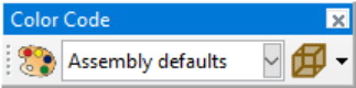
In the dropdown list of this toolbar we can select what rule does the color code follow. By default the assembly is shown in blue (‘Assembly defaults’ option), but there are many more options available: parts, instances, materials, sections, sets, element types, surfaces, faces, cells…
To color Captain America’s shield and Thor’s hammer, we will choose the “Sets” option. Then, click on the palette icon ![]() and let’s setup the color of each set. Note: sets are created with the script provided.
and let’s setup the color of each set. Note: sets are created with the script provided.
In the table, every row represents a color rule for a set. The first column “Active” indicates if the color rule applies. Colors are selected clicking on the lower right button (‘Edit color’).


In the block of code below, you can see how this process can also be automated through Python commands.
- Python
					# Display assembly on the viewport
a = mdb.models['Model-1'].rootAssembly
session.viewports['Viewport: 1'].setValues(displayedObject=a)

# Display colors through sets of geometry
cmap = session.viewports['Viewport: 1'].colorMappings['Set']

# Customize color for each set
cmap.updateOverrides(overrides={'HAMMER.ALL':(False, ),
            'HAMMER.HANDLE':(True, '#AD6756',  'Default', '#AD6756'),
            'HAMMER.HEAD':(True, '#333333', 'Default', '#333333'),
            'SHIELD.ALL':(False, ),
            'SHIELD.BLUE':(True, '#0000FF', 'Default', '#0000FF'),
            'SHIELD.CIRCLE-0':(False, ),
            'SHIELD.CIRCLE-1': (False, ),
            'SHIELD.CIRCLE-2':(False, ),
            'SHIELD.CIRCLE-3': (False, ),
            'SHIELD.RED-1':(True, '#FF0000', 'Default', '#FF0000'),
            'SHIELD.RED-2':(True, '#FF0000', 'Default', '#FF0000'),
            'SHIELD.STAR': (True, '#FFFFFF', 'Default', '#FFFFFF'),
            'SHIELD.WHITE-1':(True, '#FFFFFF', 'Default', '#FFFFFF'),})

# Refresh visualization of the colormap
session.viewports['Viewport: 1'].setColor(colorMapping=cmap)
- Lines 2 & 3: Display assembly on the viewport.
- Line 6: Create a colormap for Sets.
- Lines 9 to 21: Customize colors for each set at the assembly level.
- Line 24: Set cmap as the current colormap.
5. Generation of the full model (video)
In the following video you can see how all the steps shown above are carried out, how to use the scripts provided to generate this model and watch some results from the simulations!
And if you want to get started in Abaqus Scripting with Python check out this post to learn how to create your own scripts.
I hope that you find these tips useful!